
Transient simulation temperature field for continuous casting steel blank
 The solidification and cooling of a slab, and the simultaneous heating of the mold, is a case of transient
spatial–or three-dimensional–heat and mass transfer.
The solidification and cooling of a slab, and the simultaneous heating of the mold, is a case of transient
spatial–or three-dimensional–heat and mass transfer.
 |
Allow me to present to you our paper, which is titled: Transient simulation temperature field for continuous casting steel blank |
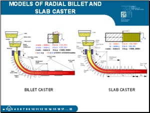 |
Here you can see a picture of a billet and slab caster A typical caster is divided into three basic sections, or parts: The first part, which is the mold, is called the primary-cooling zone. The second part, where the billet is shaped by rollers and sprayed, is called the cage, or secondary-cooling zone, and The third part, which is beyond the cage and where natural convection takes place, is called the tertiary-cooling zone. |
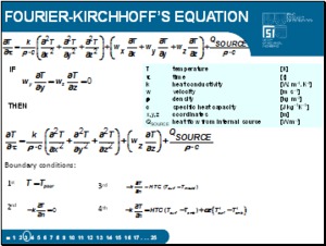 |
The solidification and cooling of a slab, and the simultaneous heating of the mold, is a case of transient spatial–or three-dimensional–heat and mass transfer. Fourier Kirchhoff’s equation, here, describes the case of continuous pouring, with the following boundary conditions: 1. The pouring temperature is the temperature at the meniscus. 2. The second condition is the adiabatic condition in the plane of symmetry. 3. The third condition is convection in the mould, and 4. The fourth condition is convection and radiation in the secondary- and tertiary-cooling zone. |
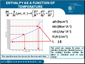 |
In this presentation we will be discussing our numerical model, which is based on the explicit difference method. In this way, it is possible to apply, more simply, the most elegant method of numerical simulation of the release of latent heat of phase or structural changes using the thermodynamic enthalpy function. This function must be known for the relevant steel. |
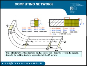 |
In order to determine the density of the network, the billet and slab were analysed in only one of its symmetrical halves - here on the right half. The selected density for our blank sizes, was: 25 unit volumes in the x-direction, 50 unit volumes in the y-direction, 2000 unit volumes in the z-direction, which is the direction of movement of the blank. The entire length of the blank in the z-directrion - from the level in the mould, down to the cutting torch, is approximately 24 to 27 meters. The mesh is generated automatically. The time step was selected within the range from 0.1 to 0.5 seconds and depends on the casting speed |
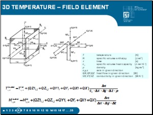 |
If the general nodal point i,j,k is positioned within the wall of the mold, then its unknown temperature in time t+Dt is given by this explicit formula: Ti,j,k = If the nodal point i,j,k is positioned within the slab, then the unknown enthalpy in time t+Dtis given by the analogical explicit formula: H i,j,k= |
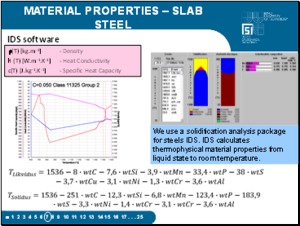 |
It is very important to set the thermo-physical and material properties of the system, including their temperature dependences. We use a solidification analysis package for steels IDS. The input data given by the user are: steel composition and the cooling rate. IDS package simulates the phase transformations during solidification and cooling and during austenite decomposition. IDS calculates thermophysical material properties from liquid state to room temperature. IDS is valid for carbon and low alloyed steels for a wide range of steel compositions as well as for stainless steels. The calculated material properties include: enthalpy, specific heat, density, conductivity, thermal contraction, solid fractions, etc. The model has been validated with numerous experiments of solidification. These properties can be set either via a table. For example, you can see the courses of heat conductivity k, specific heat capacity c and density r–of the slab steel in dependence on temperature. |
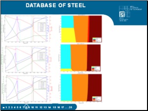 |
Dynamic solidification model has a database of properties of all cast steel. |
 |
The next step is the setting of boundary conditions, which are the heat transfer coefficients on all caster boundaries and their dependences on temperature and other operational parameters. The definition of the boundary conditions is the most difficult part of the investigation. |
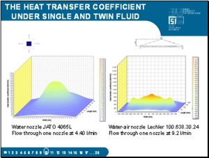 |
Heat-transfer coefficients obtained in this way are entered into a database of boundary conditions from which the model determines the appropriate heat-transfer coefficient beneath the nozzle for the required temperature of the surface of the blank, the operational flow of the water and for the required casting speed. Figures present the measured values of the heat transfer coefficients of water nozzle JATO and water-air nozzle Lechler processed by the temperature model software. |
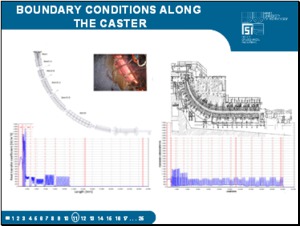 |
Figure shows the courses of the resultant heat transfer coefficients along the small radius of the caster. On a specific billet caster, the nozzles of the secondary cooling are divided into six independent regulation zones. On a specific slab caster, the nozzles of the secondary cooling are divided into 13 independent regulation zones, which enable the formation of the temperature field of the slab. |
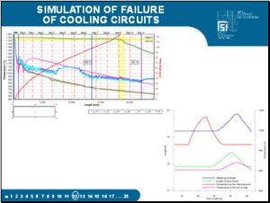 |
Figures show the output from a simulation of failure 8 and 9 circuits of the secondary cooling using the dynamic model on the analysis of the functioning of the secondary cooling. If there had really been such a failure, the temperature model would have warned the operator in time for him to decide what action to take. |
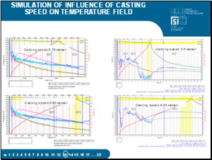 |
The casting speed is a basic technological parameter. In calculations, whose results are represented here, the operating range of the speed is considered 0.7 to 0.85 m/min for slab caster and 2 to 4 m/min for billet. The flow of water through the secondary-cooling zone, according to the technological regulations, increases linearly. The other input parameters are again left constant. |
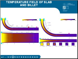 |
Here we compare the temperature field of slab and billet continuous casting. Yellow is the color of liquid steel, the red is mushy zone and blue is solid steel. |
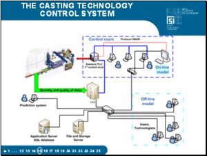 |
Figure illustrates a specific case of integration of models into the casting technology control system of a caster for the casting of steel and the quality system for slab casting at EVRAZ VITKOVICE STEEL. The caster control room is equipped with a two-processor workstation where the on-line dynamic model is running nonstop and which receives data from the 1st and 2nd levels of control via an interface program. |
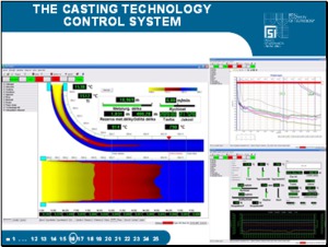 |
The input data are verified, the erroneous data being filtered out and the temperature field calculated. On the computer monitor, the operator can select from the various forms of output. According to the results, the on-line model makes recommendations for the operator in order to facilitate the control of the concasting process. |
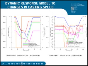 |
The left figure illustrates a testing case of a step change in the casting speed from 0.8 to 0.5 m/min and back. Such step decreases in speed can be caused by an intervention of the breakout system. The return to the original speed in reality happens more slowly and it is the dynamic model that makes it possible to find the optimal method for controlling the speed and secondary cooling. The right figure shows an example of real data from the dynamic model of a 1530×180 mm slab upon the intervention of the breakout system. This intervention brought about a drop in the casting speed from 1.22 to 0.5 m/min and an increase back to the original value. |
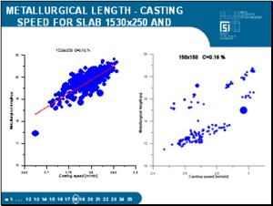 |
Figures monitored quantity is shown in dependence on the casting speed where each melt is indicated by a blue bubble whose radius corresponds to one standard deviation of the relevant quantity. The left figure is for the slab caster and the right figure is pro billet for two settings of the secondary cooling. |
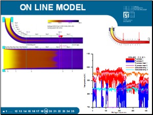 |
Figure compares the average values of the measured surface temperatures in two points with the average calculated temperatures in the same points. One point is one melt.
The graphs indicate that the measured and calculated values are practically identical in terms of their trends. |
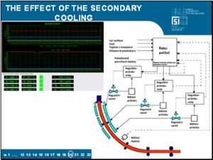 |
The setting of the secondary cooling and its optimization is a very complicated problem. |
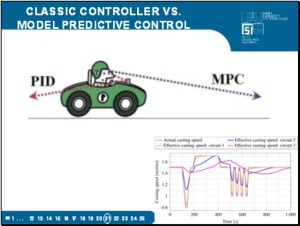 |
Model predictive control responds to the predicted future value of control deviations. PID only on current and past values. Use PID is like driving a car by looking in the rearview mirror. |
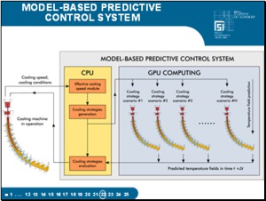 |
When using Model-based predictive control system is counted more temperature fields for fares cooling scenarios from which the selection criteria optimal. |
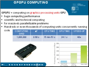 |
GPGPU = computing on graphics processing units GPU • huge computing performance • scientific and technical computing, by software CUDA • for massively parallelizable problems • Hundreds or even thousands of computing units concurrently running code |
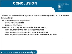 |
3D numerical model of the transient temperature field for concasting of steel is in the form of in-house software. This software has been implemented in EVRAZ VITKOVICE STEEL and TRINECKE ZELEZARNY in Czech Republic. Three ways of utilizing the results of the dynamic model: • Simulate and monitor the current temperature field • Simulate and monitor the quantities in the form of trends • Simulate and monitor the statistical quantities from individual melts |
 |
That is all for the actual presentation, … Thank you for your attention. |